The Problem
Let $\mathcal{T}$ be a triangulation of a polygonal domain $\Omega \subseteq \R^2$, and $V_h=\left\{v \in C^0(\bar{\Omega}):v|_T \text{ is linear for all } T \in \mathcal{T}\right\}$.
Let $u \in H^2(\Omega)$ and $\I u \in V_h$ be the linear interpolant of $u$. Show that
$$ \norm{u-\I u}_{L^2(\Omega)}+h\abs{u-\I u}_{H^1(\Omega)} \leq \zeta(\theta) h^2 \abs{u}_{H^2(\Omega)} $$where $h=\max _{T \in \mathcal{T}} \diam(T)$, $\theta$ is the maximum angle in $\mathcal{T}$, and $\zeta$ is an increasing positive function defined on $[\pi / 3, \pi)$.
This problem is taken from Brenner & Scott, The Mathematical Theory of Finite Element Methods, pp. 126, exercise 4.x.12.
Remark. A Maximum Angle Condition asks that the maximum angle in the triangulation stays away from $\pi$. This is different from the minimal angle condition, which asks that the minimum angle in the triangulation stays away from $0$. But the minimum angle condition implies the maximum angle condition.
Step 1
We will first treat the $L^2$ term. The interesting (and perhaps counter-intuitive) result in Finite Element theory is that the $L^2$ interpolation error does not depend on the shape regularity or the maximum angle condition. It depends only on the diameter of the element $h$.
The dependence on the maximum angle arises solely from the transformation of the gradient (the $H^1$ seminorm) back to the physical element, which we will treat in Step 2.
Geometric Setup and Coordinate Transformation
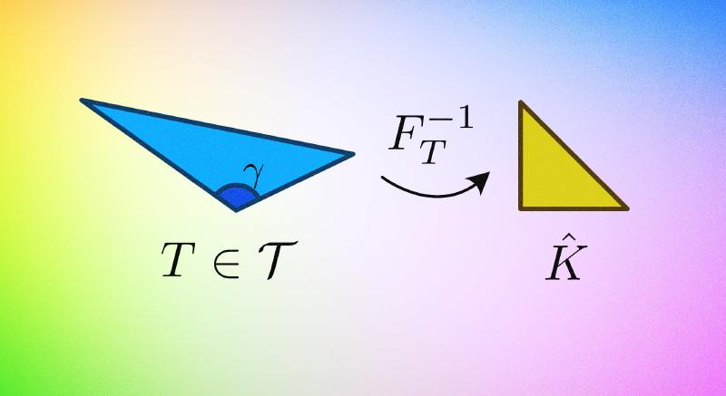
Let $T \in \mathcal{T}$ be an arbitrary triangle with vertices $P_0, P_1, P_2$. Assume without loss of generality that the angle at $P_0$, denoted by $\gamma$, is the maximum angle of $T$. Thus $\gamma \in [\pi/3, \pi)$.
Let $\hat{K}$ be the reference triangle with vertices $\hat{z}_0=(0,0)$, $\hat{z}_1=(1,0)$, and $\hat{z}_2=(0,1)$. We define the affine mapping $F: \hat{K} \to T$ by:
$$ x = F(\hat{x}) = P_0 + B\hat{x}, \quad \text{where } B = [v_1, v_2] \in \mathbb{R}^{2\times 2} $$Here, $v_1 = P_1 - P_0$ and $v_2 = P_2 - P_0$ are the edge vectors emanating from $P_0$. Let $h_1 = |v_1|$ and $h_2 = |v_2|$. Note that the diameter $h_T \simeq \max(h_1, h_2)$.
The Jacobian determinant is $J = \det(B) = h_1 h_2 \sin \gamma$.
Let $u \in H^2(T)$ and $\hat{u} = u \circ F \in H^2(\hat{K})$. Let $\mathcal{I}$ and $\hat{\mathcal{I}}$ be the linear Lagrange interpolation operators on $T$ and $\hat{K}$ respectively. By affine invariance, $\widehat{\mathcal{I}u} = \hat{\mathcal{I}}\hat{u}$. Let $e = u - \mathcal{I}u$ and $\hat{e} = \hat{u} - \hat{\mathcal{I}}\hat{u}$.
Transformation to Reference Element
We transform the $L^2$ integral from the physical triangle $T$ to the reference triangle $\hat{K}$ using the change of variables $x = F(\hat{x})$ and $dx = |\det B| d\hat{x}$.
$$ \|e\|_{L^2(T)}^2 = \int_T |e(x)|^2 dx = |\det B| \int_{\hat{K}} |\hat{e}(\hat{x})|^2 d\hat{x} = |\det B| \|\hat{e}\|_{L^2(\hat{K})}^2 \tag{1} $$On the fixed reference domain $\hat{K}$, the shape is regular. We can apply the standard interpolation error estimates.
$$ \|\hat{e}\|_{L^2(\hat{K})} = \|\hat{u} - \hat{\mathcal{I}}\hat{u}\|_{L^2(\hat{K})} \leq C_{ref} |\hat{u}|_{H^2(\hat{K})} \tag{2} $$Note that $C_{ref}$ is a universal constant depending only on the reference triangle $\hat{K}$.
Mapping the Seminorm Forward
We need to bound $|\hat{u}|_{H^2(\hat{K})}$ in terms of $|u|_{H^2(T)}$. By the chain rule, for any $i, j \in \{1, 2\}$:
$$ \frac{\partial^2 \hat{u}}{\partial \hat{x}_i \partial \hat{x}_j}(\hat{x}) = \sum_{k,l=1}^2 \frac{\partial x_k}{\partial \hat{x}_i} \frac{\partial x_l}{\partial \hat{x}_j} \frac{\partial^2 u}{\partial x_k \partial x_l}(F(\hat{x})) $$Recall that $\frac{\partial x}{\partial \hat{x}_i}$ is simply the $i$-th column of the matrix $B$, which corresponds to the edge vector $v_i$. In vector notation:
$$ \partial_{\hat{x}_i \hat{x}_j} \hat{u} = v_i^T (\nabla^2 u) v_j $$Taking the Euclidean norm (Frobenius norm for the Hessian matrix):
$$ |\partial_{\hat{x}_i \hat{x}_j} \hat{u}| \leq |v_i| |v_j| \norm{\nabla^2 u}_F \leq h^2 \norm{\nabla^2 u}_F $$where $h = \max(|v_1|, |v_2|)$ is the diameter of $T$.
Now, integrate over $\hat{K}$:
$$ \begin{aligned} |\hat{u}|_{H^2(\hat{K})}^2 &= \sum_{i,j} \int_{\hat{K}} |\partial_{\hat{x}_i \hat{x}_j} \hat{u}|^2 d\hat{x} \\ &\leq \sum_{i,j} \int_{\hat{K}} h^4 \norm{\nabla^2 u(F(\hat{x}))}_F^2 d\hat{x} \\ &= 4 h^4 \int_{\hat{K}} \norm{\nabla^2 u(F(\hat{x}))}_F^2 d\hat{x} \end{aligned} $$Change variables back to $T$ (using $d\hat{x} = |\det B|^{-1} dx$):
$$ |\hat{u}|_{H^2(\hat{K})}^2 \leq 4 h^4 |\det B|^{-1} |u|_{H^2(T)}^2 \tag{3} $$Combining the Bounds
Substitute (3) into (2), and then the result into (1):
$$ \begin{aligned} \|e\|_{L^2(T)}^2 &= |\det B| \|\hat{e}\|_{L^2(\hat{K})}^2 \\ &\leq |\det B| C_{ref}^2 |\hat{u}|_{H^2(\hat{K})}^2 \\ &\leq |\det B| C_{ref}^2 \left( 4 h^4 |\det B|^{-1} |u|_{H^2(T)}^2 \right) \end{aligned} $$Taking the square root:
$$ \|u - \mathcal{I}u\|_{L^2(T)} \leq C h^2 |u|_{H^2(T)}. $$Step 2
We will prove that for each triangle $T \in \mathcal{T}$, we have
$$ \abs{u - \I u}_{H^1(T)} \leq \frac{C}{\sin^2 \gamma} h_T \abs{u}_{H^2(T)} $$where $h_T = \diam(T)$ and $\gamma$ is the maximum angle in $T$.
Gradient Decomposition
We need to bound $\|\nabla e\|_{L^2(T)}$. The gradient $\nabla e$ is a vector in $\mathbb{R}^2$. It is convenient to decompose it along the directions of the edges $v_1$ and $v_2$, even though they are not orthogonal.
The directional derivative along $v_i$ is given by $\partial_{v_i} e = (\nabla e) \cdot v_i$. By the chain rule, this corresponds exactly to the partial derivatives on the reference element:
$$ \partial_{v_1} e(x) = \frac{\partial \hat{e}}{\partial \hat{x}_1}(\hat{x}), \quad \partial_{v_2} e(x) = \frac{\partial \hat{e}}{\partial \hat{x}_2}(\hat{x}). $$For any vector $\mathbf{w} \in \mathbb{R}^2$ and linearly independent vectors $v_1, v_2$ with angle $\gamma$ between them and lengths $h_1, h_2$:
$$ |\mathbf{w}|^2 \leq \frac{C}{\sin^2 \gamma} \left( \frac{|\mathbf{w} \cdot v_1|^2}{h_1^2} + \frac{|\mathbf{w} \cdot v_2|^2}{h_2^2} \right). $$Proof
Applying this to $\mathbf{w} = \nabla e$:
$$ |\nabla e(x)|^2 \leq \frac{C}{\sin^2 \gamma} \left( \frac{1}{h_1^2} |\partial_{v_1} e|^2 + \frac{1}{h_2^2} |\partial_{v_2} e|^2 \right). $$Transformation to Reference Element
Integrate over $T$:
$$ \|\nabla e\|_{L^2(T)}^2 \leq \frac{C}{\sin^2 \gamma} \left( \frac{1}{h_1^2} \|\partial_{v_1} e\|_{L^2(T)}^2 + \frac{1}{h_2^2} \|\partial_{v_2} e\|_{L^2(T)}^2 \right). $$Transform the integrals to $\hat{K}$ using $dx = |\det B| d\hat{x}$:
$$ \|\partial_{v_1} e\|_{L^2(T)}^2 = |\det B| \, \|\partial_{\hat{x}_1} \hat{e}\|_{L^2(\hat{K})}^2 $$$$ \|\partial_{v_2} e\|_{L^2(T)}^2 = |\det B| \, \|\partial_{\hat{x}_2} \hat{e}\|_{L^2(\hat{K})}^2 $$
Substituting back:
$$ \|\nabla e\|_{L^2(T)}^2 \leq \frac{C |\det B|}{\sin^2 \gamma} \left( \frac{1}{h_1^2} \|\partial_{\hat{x}_1} \hat{e}\|_{L^2(\hat{K})}^2 + \frac{1}{h_2^2} \|\partial_{\hat{x}_2} \hat{e}\|_{L^2(\hat{K})}^2 \right) \tag{4} $$Anisotropic Bounds
Let $\hat{K}$ be the reference triangle with vertices $(0,0)$, $(1,0)$ and $(0,1)$, and let $\zeta \in W^m_p(\hat{K})$ for $m \geq 2$ and $1 \leq p \leq \infty$. Then
$$ \| \partial_{x_j}(\zeta - \mathcal{I}\zeta) \|_{L^p(\hat{K})} \leq C | \partial_{x_j} \zeta |_{W^{m-1}_p(\hat{K})} $$where $\mathcal{I}\zeta$ is the interpolant of $\zeta$ in the $\mathcal{P}_{m-1}$ Lagrange finite element.
Proof
Without loss of generality, let $j=1$ and denote $x_j = x$. Let $\partial_x = \partial/\partial x$. Define $u = \partial_x \zeta$. Note that $u \in W^{m-1}_p(\hat{K})$.
The term $\partial_x (\mathcal{I}\zeta)$ is a polynomial in $\mathcal{P}_{m-2}$. We want to relate this term directly to $u = \partial_x \zeta$. To do this, we must establish that the operation $\zeta \mapsto \partial_x (\mathcal{I}\zeta)$ factors through $\partial_x \zeta$.
One can verify that if $\partial_x \zeta = 0$ (i.e., $\zeta$ is independent of $x$), then $\partial_x (\mathcal{I}\zeta) = 0$.
Given $u \in W^{m-1}_p(\hat{K})$, let $\zeta$ be any primitive such that $\partial_x \zeta = u$. Define:
$$ \Pi u := \frac{\partial}{\partial x} (\mathcal{I}\zeta) $$This definition is consistent. If $\zeta_1$ and $\zeta_2$ are two primitives of $u$, then $\partial_x(\zeta_1 - \zeta_2) = 0$. By Lemma 1, $\partial_x \mathcal{I}(\zeta_1 - \zeta_2) = 0$, implying $\partial_x \mathcal{I}\zeta_1 = \partial_x \mathcal{I}\zeta_2$.
We now check how $\Pi$ acts on polynomials. This is crucial for applying the Bramble-Hilbert lemma.
One can then verify the following: if $q \in \mathcal{P}_{m-2}$, then $\Pi q = q$.
We can now rewrite the LHS of the inequality using $u = \partial_x \zeta$:
$$ \frac{\partial}{\partial x}(\zeta - \mathcal{I}\zeta) = \partial_x \zeta - \partial_x (\mathcal{I}\zeta) = u - \Pi u = (I - \Pi)u $$We need to bound $\|(I - \Pi)u\|_{L^p(\hat{K})}$. Consider the linear operator $T = I - \Pi$.
-
Boundedness: The operator $\Pi$ is composed of integration (bounded on compact domains), interpolation (bounded $W^m_p \to W^m_p$), and differentiation. Specifically, $\Pi : W^{m-1}_p \to \mathcal{P}_{m-2}$. Since $\mathcal{P}_{m-2}$ is finite-dimensional, all norms are equivalent, and $\Pi$ is bounded on $W^{m-1}_p$. Thus, $T$ is bounded from $W^{m-1}_p(\hat{K})$ to $L^p(\hat{K})$.
-
Vanishing on Polynomials: By Lemma 2, for any $q \in \mathcal{P}_{m-2}$, $\Pi q = q$, so $T(q) = q - q = 0$. The operator vanishes on $\mathcal{P}_{m-2}$.
-
The Estimate: By the Bramble-Hilbert lemma, if a bounded linear operator $T: W^{k}_p \to L^p$ vanishes on $\mathcal{P}_{k-1}$, then:
$$ \|Tu\|_{L^p} \le C |u|_{W^{k}_p} $$Here, we set $k = m-1$. The operator vanishes on $\mathcal{P}_{m-2}$. Therefore:
$$ \|(I - \Pi)u\|_{L^p(\hat{K})} \le C |u|_{W^{m-1}_p(\hat{K})}. $$
We apply the theorem with $m=2$:
$$ \|\partial_{\hat{x}_j} \hat{e}\|_{L^2(\hat{K})} \leq C |\partial_{\hat{x}_j} \hat{u}|_{H^1(\hat{K})} $$This is an anisotropic estimate because the bound for $\partial_1$ depends only on derivatives of $\partial_1$ (i.e., $\partial_{11}$ and $\partial_{12}$), ignoring $\partial_{22}$.
For $j=1$:
$$ \|\partial_{\hat{x}_1} \hat{e}\|_{L^2(\hat{K})}^2 \leq C \left( \|\partial_{11} \hat{u}\|_{L^2(\hat{K})}^2 + \|\partial_{12} \hat{u}\|_{L^2(\hat{K})}^2 \right) \tag{5} $$For $j=2$:
$$ \|\partial_{\hat{x}_2} \hat{e}\|_{L^2(\hat{K})}^2 \leq C \left( \|\partial_{22} \hat{u}\|_{L^2(\hat{K})}^2 + \|\partial_{21} \hat{u}\|_{L^2(\hat{K})}^2 \right) \tag{6} $$Scaling Back to Physical Derivatives
As before, we use the chain rule to relate the reference Hessian to the physical Hessian:
$$ |\partial_{ij} \hat{u}| \leq |v_i| |v_j| |\nabla^2 u|_F = h_i h_j |\nabla^2 u|_F $$Integrating over $\hat{K}$ and mapping back to $T$:
$$ \|\partial_{ij} \hat{u}\|_{L^2(\hat{K})}^2 \leq \int_{\hat{K}} h_i^2 h_j^2 |\nabla^2 u(F(\hat{x}))|^2 d\hat{x} = h_i^2 h_j^2 |\det B|^{-1} |u|_{H^2(T)}^2 $$Now, substitute these into our estimates (5) and (6).
For the first term ($j=1$, divided by $h_1^2$):
$$ \begin{aligned} \frac{1}{h_1^2} \|\partial_{\hat{x}_1} \hat{e}\|^2 &\leq \frac{C}{h_1^2} \left( \|\partial_{11} \hat{u}\|^2 + \|\partial_{12} \hat{u}\|^2 \right) \\ &\leq \frac{C}{h_1^2} |\det B|^{-1} |u|_{H^2(T)}^2 \left( h_1^4 + h_1^2 h_2^2 \right) \\ &= C |\det B|^{-1} |u|_{H^2(T)}^2 \left( h_1^2 + h_2^2 \right) \end{aligned} $$For the second term ($j=2$, divided by $h_2^2$):
$$ \begin{aligned} \frac{1}{h_2^2} \|\partial_{\hat{x}_2} \hat{e}\|^2 &\leq \frac{C}{h_2^2} \left( \|\partial_{22} \hat{u}\|^2 + \|\partial_{21} \hat{u}\|^2 \right) \\ &\leq \frac{C}{h_2^2} |\det B|^{-1} |u|_{H^2(T)}^2 \left( h_2^4 + h_2^2 h_1^2 \right) \\ &= C |\det B|^{-1} |u|_{H^2(T)}^2 \left( h_2^2 + h_1^2 \right) \end{aligned} $$Final Assembly
Substitute these bounds back into equation (4):
$$ \begin{aligned} \|\nabla e\|_{L^2(T)}^2 &\leq \frac{C |\det B|}{\sin^2 \gamma} \left[ C |\det B|^{-1} |u|_{H^2(T)}^2 (h_1^2 + h_2^2) + C |\det B|^{-1} |u|_{H^2(T)}^2 (h_2^2 + h_1^2) \right] \\ &= \frac{C}{\sin^2 \gamma} (h_1^2 + h_2^2) |u|_{H^2(T)}^2 \end{aligned} $$Since $h_1^2 + h_2^2 \leq 2 h_T^2$, we have
$$ \|\nabla e\|_{L^2(T)} \leq \frac{C}{\sin \gamma} h_T |u|_{H^2(T)}. $$Step 3
Now we can put everything together by summing the local estimates over all triangles $T \in \mathcal{T}$. Let $\theta = \max_{T \in \mathcal{T}} \gamma_T$ be the maximum angle in the triangulation.
For the $L^2$ norm:
$$ \norm{u-\I u}_{L^2(\Omega)}^2 = \sum_{T \in \mathcal{T}} \norm{u-\I u}_{L^2(T)}^2 \leq \sum_{T \in \mathcal{T}} C h_T^4 \abs{u}_{H^2(T)}^2 \leq C h^4 \abs{u}_{H^2(\Omega)}^2 $$For the $H^1$ seminorm:
$$ \abs{u-\I u}_{H^1(\Omega)}^2 = \sum_{T \in \mathcal{T}} \abs{u-\I u}_{H^1(T)}^2 \leq \sum_{T \in \mathcal{T}} \frac{C}{\sin^2 \gamma_T} h_T^2 \abs{u}_{H^2(T)}^2 \leq \frac{C}{\sin^2 \theta} h^2 \abs{u}_{H^2(\Omega)}^2 $$Taking square roots yields:
$$ \norm{u-\I u}_{L^2(\Omega)} \leq C h^2 \abs{u}_{H^2(\Omega)} \quad \text{and} \quad \abs{u-\I u}_{H^1(\Omega)} \leq \frac{C}{\sin \theta} h \abs{u}_{H^2(\Omega)} $$Multiplying the $H^1$ estimate by $h$ and adding them together:
$$ \norm{u-\I u}_{L^2(\Omega)} + h \abs{u-\I u}_{H^1(\Omega)} \leq C \left( 1 + \frac{1}{\sin \theta} \right) h^2 \abs{u}_{H^2(\Omega)} $$This completes the proof, with $\zeta(\theta) = C(1 + (\sin \theta)^{-1})$.
Conclusion
The reason the Maximum Angle Condition is famous is precisely because standard Finite Element Theory (Ciarlet-Raviart) assumed the “Minimum Angle Condition” (shape regularity) to bound the Jacobian inverse $B^{-1}$.
- $L^2$ error: Only involves $B$. Never blows up for flat triangles.
- $H^1$ error: Involves $B^{-T} \nabla_{\hat{x}}$.
- Standard theory bounds $\|B^{-1}\| \le h/\rho$ (where $\rho$ is the inscribed circle radius). This blows up if the triangle is flat (anisotropic).
- Maximum angle theory notices that if the gradients align with the long edges, the derivatives don’t actually see the “short direction” (the altitude), allowing us to replace $1/\sin(\gamma_{min})$ with $1/\sin(\gamma_{max})$.